Predictive aerodynamics - Euler was right
- Real Flight Simulation in the Digital Math framework
Authors
- Johan Jansson (jjan@kth.se)
- Claes Johnson
- Ridgway Scott
Introduction
We show that computing turbulent solutions to Euler’s equations with a slip boundary condition offers a Theory of Everything ToE for slightly viscous incompressible fluid flow as a parameter-free model, covering a vast area of applications in vehicle aero/hydrodynamics including airplanes, ships and cars. This work resolves the Grand Challenges of fluid dynamics described in NASA Vision 2030.
The foundation of the methodology is an extremely efficient Direct FEM Simulation (DFS) method. We describe a breakthrough in efficiency, allowing extrenely small numerical dissipation by choosing very small stabilization coefficients, while allowing very large time step size.
This work is developed as part of the Digital Math framework [2] - as the foundation of modern science based on constructive digital mathematical computation.
We show that Euler CFD by the scientific method in Digital Math predicts drag, lift and pressure distribution in close correspondence with observations for real problems with complex geometry and so can serve to deliver complete realistic aero/hydro-data for simulators without input from model experiments in wind tunnel and towing tank or full-scale experiments, as a new revolutionary capability.
1 Euler CFD overview
The methodology is a Direct FEM Simulation (DFS) [1, 3] of the first principle Euler equations with a slip boundary condition - here denoted Euler CFD. The methodology is realized according to the scientific method in the Digital Math framework. We call this realization Real Flight Simulator (RFS).
These first principle equations are discretized by the Direct FEM approach, meaning Galerkin-Least-Squares (GLS) stabilization.
The Galerkin part of the method is formulated as below in FEniCS notation:
F_Galerkin = inner(udot + grad(u)*u + grad(p), v)*dx
F_Galerkin += inner(div(u), q)*dx
and in corresponding strong form in Latex notation:
| (1) |
An overview of the main ingredients of Euler CFD with the Digital Math RFS realization are given below, a more detailed description is in section 6:
Free slip boundary condition with 3D rotational slip separation
No thin boundary layers to resolve.
We show that the flow can separate with 3D rotational slip separation, at high velocity. See the 3D cylinder benchmark below for an illustration.
Our detailed validation of the reference benchmarks in the field: HiLiftPW2-4, NACA0012 wing, etc. all show that with only the pressure drag our results are within 5% of the experiment. This means skin friction drag is a small/negligible effect, which either can be omitted, or added as a minor adjustment.
In [4] we give an overview of both experimental and Euler CFD evidence, of low dependence of drag from Reynolds number in untripped configurations, consistent with free slip, from e.g. Abbott.
Automatic turbulence modeling by residual stabilisation
Through weighted least squares residual stabilisation generating turbulent dissipation , as a solution to the open problem of turbulence modeling [?]. In particular, the weighted strong residual measures the turbulent dissipation as a mesh independent quantity meeting Kolmogorov’s K41 conjecture of finite turbulent dissipation [72].
Adaptive adjoint-based a posteriori error control
Guaranteeing mesh-independence of drag and lift, and accuracy to a few percent in the validations.
Reproducibility
Guaranteeing the scientific method, allowing inspection, falsification, modification.
There is today a reproducibility crisis in science which we resolve with the Digital Math framework, and specifically here for Euler CFD with RFS.
Automated Digital Math
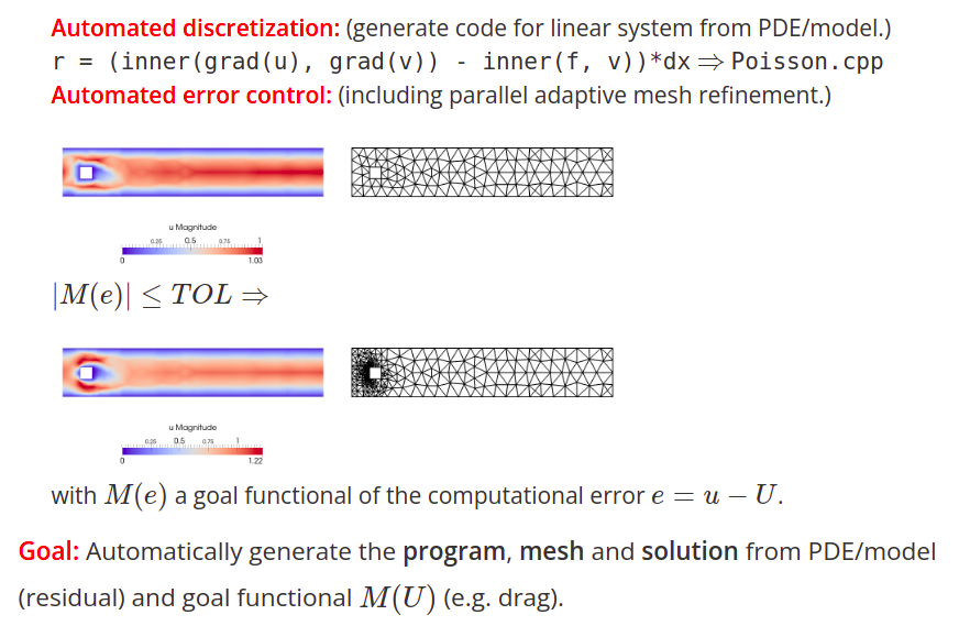
We leverage our Open Source FEniCS framework, which automated the solution of partial differential equations by FEM, taking the mathematical notation as input. This allows an automation of Digital Math, described in a bird’s eye view below:
1.1 Extremely efficient stabilized Direct FEM
The predictive adaptive stabilized Direct FEM Simulation method takes the form:
F = F_Galerkin + F_Stab
where F˙Stab is a residual-based Least Squares Galerkin stabilization of the form with proportional to the mesh size h, controlled by the duality-based adaptive error control.
F_Stab provides numerical dissipation for the unresolved subscales in a Direct predictive and adaptive setting.
In previous work on DFS we have chosen or with . In this work we show a key breakthrough, choosing for the velocity component U and for the pressure component P. This corresponds to an efficiency increase of many orders of magnitude, which is key for the resolution of the Grand Challenges in fluid dynamics.
2 Validation
2.1 High Lift Prediction Workshop 4


2.2 NACA0012 wing at aoa=0
We can now present breakthrough results validating RFS for the NACA0012 aoa=0 case, demonstrating that RFS predicts the regime of cruising aircraft and ships (hydrodynamics).
3 Euler CFD as a solution to NASA Vision 2030
We see that Euler CFD with the Real Flight Simulator (RFS) realization already today in 2021 satisfies the goals of the NASA Vision 2030 challenges:
1. Emphasis on physics-based, predictive modeling
Euler/RFS is predictive by being first-principles, parameter-free and mesh/discretization independent by adjoint-based adaptive error control.
2. Management of errors and uncertainties resulting from all possible sources
Euler is first-principles, and does not have explicit modeling parameters. RFS relies on adjoint-based adaptive error control to guarantee mesh/discretization-independence, and additionally automatically generates the low-level source code from mathematical notation (just a few lines), thus eliminating the possibility of human bugs.
3. A much higher degree of automation in all steps of the analysis process
RFS relies on automated mesh generation based on adjoint-based adaptive error control, and additionally automatically generates the low-level source code from mathematical notation (just a few lines) including the adjoint formulation and the adjoint solution.
4. Ability to effectively utilize massively parallel, heterogeneous, and fault-tolerant HPC architectures
We demontrate that Euler/RFS has extremely cheap and fast performance ( 200 core hours), which allows an extreme effectiveness by being able to run a large number of simulations on in principle any parallel computer (also e.g. any virtual machine in a cloud setting, even in a web browser), at a cost affordable to any engineer, researcher or even student.
5. Flexibility to tackle capability- and capacity-computing tasks in both industrial and research environments:
The same answer as above. We demontrate that Euler/RFS has extremely cheap and fast performance ( 200 core hours), which allows an extreme effectiveness by being able to run a large number of simulations on in principle any parallel computer (also e.g. any virtual machine in a cloud setting, even in a web browser), at a cost affordable to any engineer, researcher or even student.
6. Seamless integration with multidisciplinary analyses that will be the norm in 2030
Euler/RFS is realized in the Digital Math framework in FEniCS, taking the mathematical notation (just a few lines) as input and automatically generating the low-level source code. We have demonstrated general fluid-strucure interaction (FSI) generalizations in a very simple and automated way, and other multidisciplinary generalizations are possible or have been done in a similar way. Digital Math means an Open Source setting, where it’s easy and natural to merge and integrate different formulations for e.g. different physical phenomena.
4 Euler’s Dream
Read Euler, read Euler, he is the master of us all. (Laplace)
In 1755 the German mathematician Euler formulated a mathematical model describing the flow of air (subsonic) and water with the following prophetic declaration of Euler’s Dream [23]:
- My two equations contain all of the theory of fluid mechanics. It is not the principles of mechanics we lack to pursue this analysis but only Analysis (computation), which is not sufficiently developed for this purpose.
These are Euler’s equations for (unit density) slightly viscous incompressible fluid flow formulated in terms of fluid velocity and fluid pressure depending on space-time coordinates as an expression of force balance (Newton’s 2nd Law) and incompressibility complemented by a slip boundary condition. They read [16]:
| (2) |
where is a spatial domain occupied by the fluid with boundary with unit normal acting like a solid wall impenetrable to the fluid as expressed by . The only forces acting on the fluid (without gravitation) are the internal pressure gradient as a volume force in combined with a surface pressure force from the wall acting in the normal direction on . Formally there are no internal viscous shear forces (zero viscosity) and no force tangential to the boundary (zero skin friction).
In bluff body flow is the domain filled by fluid flowing past a volume occupied by a solid body at rest in a coordinate system with the flow velocity being constant at large distance from the body as a far-field condition. The basic problem in bluff body flow is to determine the pressure distribution from the fluid on the body with drag and lift as net forces opposite and perpendicular to the main flow direction in normalized form appearing as coefficients of drag and and lift . This is the basic problem of vehicle aero/hydrodynamics including airplanes, ships and cars. We shall see that computing turbulent solutions of Euler’s equations allows accurate prediction of drag and lift for a body of arbirtary shape, as a realisation of Euler’s Dream by computing.
As is clear from (2) the Euler equations are parameter-free since viscosity and skin friction parameters are set to zero. This means that the Euler equations/Euler’s Dream represent Einstein’s ideal mathematical model as a Theory of Everything ToE for a certain range of physics (slightly viscous incompressible) flow, that is a mathematical theory capable of making predictions about reality (drag and lift) without any input of parameters such as viscosity and skin friction. We give below massive evidence that computation of turbulent solutions to Euler’s equations is a ToE for fluid mechanics, and as such very remarkable and useful. But it took 250 years to make computing powerful enough to make Euler’s Dream come true, and the start for Euler in 1755 was rocky.
Eulers French adversary mathematician d’Alembert namely quickly crushed Euler’s grand plan by showing that Euler’s equations admitted certain solutions (potential solutions) showing zero drag and lift of a body moving through air or water, in direct contradiction to observation [22, 32, 33, 29]. This was coined d’Alembert’s Paradox (in fact realised by Euler before 1755 [33]), which from start as expressed by Chemistry Nobel Laureate Hinshelwood, separated practical fluid mechanics (hydraulics) describing phenomena (drag, lift), which cannot be explained, from theoretical fluid mechanics explaining phenomena (zero drag, lift), which cannot be observed.
The paradox showed to resist all attempts of resolution by numbers of most able mathematicians, but zero lift is in particular incompatible with flight, and so had to be resolved at the dawn to modernity when powered human flight was shown to be possible by the Wright brothers in 1903. The young ambitious fluid mechanician Ludwig Prandtl took on the challenge by presenting a resolution in a 10 minute presentation at a 1904 mathematics conference at Heidelberg of a sketchy 8-page note On flow motion with very small viscosity [59, 26, 8]. Prandtl discriminated potential flow with zero skin friction claiming that a real fluid always meets a solid wall through a boundary layer with zero tangential relative velocity named no-slip, then apparently as a result of sufficient skin friction supposed to cause ”flow separation by adverse pressure” and drag. Prandtl thus ”resolved” d’Alembert’s Paradox by declaring that the Euler equations with slip had to be expanded to the Navier-Stokes equations including boundary layer effects from positive viscosity with in particular a no-slip boundary condition as somehow an effect of viscosity, although admittedly ”very small”. But no-slip was an ad hoc assumption which Prandtl could not justify, since the exact nature of the microscopic or effective macroscopic contact between fluid and wall was unknown to him and so has remained into our days.
Prandt started out boldly declaring I have now set myself the task to investigate systematically the laws of motion of a fluid whose viscosity is very small [59] (same as Euler) with the plan of showing a big effect (substantial drag and lift) from a very small cause (very small viscosity), however as scientific problem something very delicate by asking for very detailed analysis. Large scale instability is a different thing.
Navier-Stokes equations as presented by Navier in 1823 (clarified by Saint-Venant 1930 [69] and Stokes [65] in 1842) were combined with a slip-friction boundary condition (shown below) and so Prandtl’s no-slip was by no means a necessity, only a convenient assumption (to get rid of potential flow) as expressed by Prandtl [59]:
- By far the most important question in the problem area is the behaviour of fluids at the walls of solid bodies. One does sufficient justice to the physical processes in the boundary layer between the fluid and the solid body if one assumes that the fluid adheres to the wall and that the velocity there is zero or correspondingly equal to the velocity of the body.
Anyway, the fluid mechanics community was with the help of Prandtl relieved from a seemingly unresolvable most disturbing paradox as expressed by Hinshelwood, and so Prandtl in the 1920s was named Father of Modern Fluid Mechanics [61, 67] based on the Navier-Stokes equations with no-slip and not Euler’s equations with slip.
But there was one main caveat: The Navier-Stokes equations with no-slip have solutions with boundary layers so thin that computational resolution is impossible with any forseeable computational power [52]. Prandtl’s resolution thus came with the cost of making Computational Fluid Dynamics CFD into an impossibility asking for resolution of atomistic scales in a macroscopic setting, or complicated modeling.
In 2010, Hoffman and Johnson published [40] a different resolution of d’Alembert’s Paradox showing that the reason zero-drag/lift of potential flow cannot be observed, is that potential flow as gradient of a potential satisfying Laplace’s equation, is large scale unstable at separation as exact solution to Euler’s equations, and so is replaced by solution with a turbulent wake after separation with drag/lift. In this article we now present Digital Math reproducible proof of this resolution, by computing turbulent solutions to Eulers equations with slip from a principle of best possible approximate solution with drag and lift in close agreement with observations, supported by mathematical analysis [38, 39]. Here large scale instability is not a small cause in the same sense as very small viscosity, and so is open to mathematical understanding. The new resolution was anticipated by Euler expecting separation being different from attachement [33, 56].
As a spin off a New Theory of Flight [37, 36] was developed revealing the true Secret of Flight [70] in physical terms, very different from the unphysical lifting line theory advocated by Prandtl as a follow up of the unhysical Kutta-Zhukowski circulation theory [15].
In 2017 Johan Jansson et. al. finally resolved the NASA Vision 2030 grand challenge by completing the methodology, and with Digital Math demonstrated prediction of stall in the Third High Lift Prediction Workshop [3]. Jansson showing that the critical addition of noise guaranteed the triggering of the instabilities in the 3D slip separation mechanism.
Stokes [65] suggested the possibility that a given flow motion does not imply its necessity [29] as expression of instability: There may even be no steady mode of motion possible, in which case the fluid would continue perpetually eddying. This was shown to be a reality in the new resolution 2010 of d’Alembert’s Paradox. Stokes idea was expressed by the mathematician Garrett Birkhoff in the 1st edition 1950 of his Hydrodynamics [14], but was removed in the 2nd edition because of harsh critcism from the fluid dynamics community and so only managed to resurface 55 years after Prandtl’s death in the new resolution.
Darrigol [29] (also [6]) gives a detailed exposition of early work on hydrodynamic stability by Stokes, Helmholtz, Lord Kelvin and Reynolds, as well as attempts to resolve d’Alembert’s paradox by Rayleigh, Poncelet and Saint-Venant followed by that by Father Prandtl, which became the resolution serving the modern fluid mechanics of the 20th century, although: In summary, Prandtl’s early insights into boundary-layer theory did not bring him much closer to a practical solution of low-viscosity resistance problems. The difficulties of the determination of separated flow remain unsolved to this day.
We now present massive evidence collected in this article in Digital Math reproducible form showing that computing turbulent solutions of Euler’s equations with slip, which we will refer to as Euler CFD, opens basically all of slightly viscous nearly incompressible flow to predictive simulation without parameter input and need to resolve thin no-slip boundary layers, thus with readily available computing power, all along Euler’s visionary prophecy.
Euler thus was right in predicting that his dream would come true once the computing power (Analysis) was strong enough to compute turbulent solutions of the Euler equations with slip, and Prandtl was wrong claiming drag and lift to be effects of unresolvable thin no-slip boundary layers making CFD into an impossibility. It took 250 years, but now it is here and sets a new standard in engineering by computational mathematics opening a window to the Clay Millennium Problem on Navier-Stokes equations [17] presented as follows:Mathematicians and physicists believe that an explanation for and the prediction of both the breeze and the turbulence can be found through an understanding of solutions to the Navier-Stokes equations. Although these equations were written down in the 19th Century, our understanding of them remains minimal. The challenge is to make substantial progress toward a mathematical theory which will unlock the secrets hidden in the Navier-Stokes equations. It seems that the secrets were hidden already in the Euler equations and can now be revealed by Euler CFD.
5 Digital Math: Scientific Automated Flow Simulation
The scientific process has not kept up with digital technology, and there is today a reproducibility crisis. Lorena Barba representing NASEM describes the situation as:
“The widespread use of computation and large volumes of data have transformed most disciplines of science and enabled new and important discoveries. But this revolution is not yet reflected in the ways that scientific findings are published and shared with the relevant communities. Extending the scholarly record to data, software, and computational environments and workflows is a must to ensure the robustness of science in this digital era.”
We present the Digital Math framework as the foundation for modern science based on constructive digital mathematical computation, and as a solution to the reproducbility crisis. The computed result (coefficient vector, FEM function, plot, etc.) is a mathematical theorem, and the mathematical Open Source code, here in the FEniCS framework, and computation is the mathematical proof. We can also derive additional constructive proofs from the FEniCS and FEM formulation, such as stability.
Digital Math represents digitalization of science, mathematics, society and industry in the form of automated and easily understandable computation of mathematical models. It is here realized in the Open Source FEniCS framework with world-leading performance and recognized at the highest level of science and industry together with an effective pedagogical concept with combined abstract theory and mathematical interactive programming in a ”one-click” cloud-HPC web-interface, accessible to anyone: Here is the full adaptive Euler CFD methodology for a standard 3D cube benchmark case [2] for you to inspect, run, modify, and reproduce, just as all examples presented.
https://colab.research.google.com/github/johanjan/MOOC-HPFEM-source/blob/master/DigiMat˙Pro˙Fluid˙3D˙adaptive˙cube.ipynb
Computational solution of turbulent solutions of Euler’s equations as Euler CFD is automated using FEniCS [30] for automation of the finite element discretisation used to express the principle of best possible approximate solution. This brings a new tool of Automated Flow Simulation with only geometry input, which in particular allows for the first time computation of complete aero-data (forces) for any given airplane/car/ship for design, Digital Twins, interactive simulators, etc. Euler CFD can include (small) positive boundary friction allowing also flow before drag crisis to be computed, but it introduces friction as a coefficient to be fittted to experiments. For high Reynolds number beyond drag crisis - the regime relevant to aerodynamics - this is not needed, and Euler CFD is completely parameter-free.
6 Euler CFD: Turbulent Solutions of Euler’s Equations
When I meet God, I am going to ask him two questions: why relativity? And why turbulence? I really believe he will have an answer for the first. (Heisenberg)
Turbulent solutions to Euler’s equations as Euler CFD are computed as best possible approximate solutions in the sense of having residuals which are small in a weak sense and not too large in a strong and sense, in a situation when all solutions with small strong residuals (laminar solutions and potential solutions in particular) are unstable (as solutions to Euler’s equations) and thus do not persist over time. We here face a new situation where only turbulent flow is computable and laminar not, as an expression of the fluctuating nature of turbulence as a consequence of local exponential instability, as seen in a waving flag showing the only motion which can persist.
More precisely, the best possible aspect is realised by a finite element method augmenting small weak residuals from Galerkin orthogonality with weighted least squares control of strong residuals, the latter introducing a viscous effect as a form of turbulent viscosity set by computation alone without need to model or measure turbulent viscosity beyond human comprehension. It connects to Leibniz idea of the Real World as a Best Possible World; the flag is doing its best possible as well as Euler CFD showing mesh-independence of drag and lift with readily available computing power.
Euler CFD takes the following space-discrete variational form: Find such that for , for all
| (3) |
where denote inner products, and are finite element spaces of continuous piecewise linear velocity-pressure functions satisfying and on and appropriate far-field conditions, local finite element size, and and are constants chosen from a principle of best possible with respect to output measured by the solution to an associated linearised dual problem. Time stepping is performed using continuous piecewise linear trial functions and piecewise constant test functions in time (Crank-Nicolson type). Euler CFD shows insensitivity within quite wide margins to the precise choice of and , as well as mesh size once small enough to resolve geometry and separation.
Euler CFD performs automatic turbulence modeling through weighted least squares residual stabilisation of the momentum equation combined with pressure stabilisation with corresponding turbulent dissipation obtained choosing in (3):
| (4) |
with as a representative part of the full momentum residual when not small. Turbulence is then identified by substantial turbulent dissipation over time (showing mesh size independence) as an expression of impossbility of computing a solution over time with small momentum residual in a strong () sense and in regions of turbulence.
Residual stabilisation of the momentum equation is necessary because weak satisfaction in the form for all smooth , does not itself give control of the kinetic energy , the reason being that it is not feasible to choose because is not smooth.
Euler CFD includes adaptive duality based a posteriori error control guaranteeing drag and lift up to a few percent. A key element is here the oscillating character of turbulent flow leading to cancellation in the linearised dual problem making the dual solution computable and properly bounded [38].
Euler CFD includes automatic turbulence modeling through weighted strong residual control as a dissipative effect with a complex flow dependence beyond viscous shear stress. It appears as a solution to the open problem of turbulence modeling [?]. In particular, the weighted strong residual measures the turbulent dissipation as a mesh independent quantity meeting Kolmogorov’s K41 conjecture of finite turbulent dissipation [72].
7 Predictive Euler CFD - Resolution of the paradox
We show that predictive Euler CFD resolves the paradox. The potential solution with zero drag is unstable - shown by stability analysis and computational evidence with adaptive error control. We illustrate the resolution by the basic cylinder model problem, and also by the most advanced benchmark in the world representing vehicles and aerodynamic devices - the High Lift Prediction Workshop, where we show that Euler CFD predicts the experiment to 5% with mesh independence, and predicts they key stall mechanism.
In Figure 14 we show our resolution of the paradox with Digital Math Euler CFD: the potential solution is unstable and develops streamwise vortices on the downstream side of the cylinder, generating “3D slip separation” - separation at high flow velocity.
In Figures 7 and 8 we show prediction of stall in the Third High Lift Prediction Workshop [3], both CD and CL within 5% of the experiment and mesh-independent (the experimental drag had a systemic error of appx. 10%). This represents the resolution of the NASA Vision 2030 grand challenge by completing the methodology with the critical addition of noise guaranteeing the triggering of the instabilities in the 3D slip separation mechanism., and with Digital Math guaranteeing the scientific method.
7.1 Car benchmark - DrivAer
7.2 Wing benchmark - NACA0012
7.3 Cylinder benchmark - 3D slip separation
8 Conclusions
We have showed that computing turbulent solutions to Euler’s equations with a slip boundary condition offers a Theory of Everything ToE for slightly viscous incompressible fluid flow as a parameter-free model, we are now able to predict a vast area of applications in vehicle aero/hydrodynamics including airplanes, ships and cars. This work resolves the Grand Challenges of fluid dynamics described in NASA Vision 2030.
Key specific results are breakthrough results validating RFS for the High Lift Prediction Workshops and the NACA0012 aoa=0 case, demonstrating that RFS predicts the regime of cruising aircraft and ships (hydrodynamics). Additionally we show Digital Math simulations of similar applications such as the full car DrivAer automotive standard benchmark, etc.
9 Digital Math: Reproducible results and open source software
The software for reproducing the results in the paper is available as part of the distribution for the Digital Math framework.
Contact Johan Jansson (jjan@kth.se) for instrutions how to run the software in a Google Cloud virtual machine in an easy web interface (free credits).
References
[1] http://digimat.tech/digimat/#digimat-Pro
[2] https://colab.research.google.com/github/johanjan/MOOC-HPFEM-source/blob/master/DigiMat_Pro_Fluid_3D_adaptive_cube.ipynb
[3] J. Jansson et. al., Time-resolved adaptive direct fem simulation of high-lift aircraft configurations. Springer Brief: Numerical simulation of the aerodynamics of high-lift configurations, 2017.
[4] Johan Jansson, Claes Johnson, Ridgway Scott, Massimiliano Leoni, Tamara Dancheva, Ezhimathi Krishnasamy, Rahul Kumar, World-unique Direct FEM prediction of drag - opening new paradigm for aircraft and general design, preprint, 2019 http://www.csc.kth.se/~jjan/publications/dfs-flight-drag_preprint_2019-11-10_02.pdf
[5] A. A. Abdel-Rahman, W. Chakroun, Wind Engineering 21(3):125-137, Jan 1997.
[6] J. A. D. Ackroyd, B. P. Axcell and A.L. Ruban, Early Developments in Modern Aerodynamics, Butterworth.Heinemann, 2001.
[7] J. D. Anderson, A History of Aerodynamics and Its Impact on Flying Machins, Cambridge University Press, 1997.
[8] J. D. Anderson, Ludwig Prandtl’s Boundary Layer, Physics Today, Dec 2005.
[9] 3rd AIAA CFD High Lift Prediction Workshop, 2017, https://hiliftpw.larc.nasa.gov/index-workshop3.html.
[10] 6th AIAA CFD Drag Prediction Workshop 2016, https://aiaa-dpw.larc.nasa.gov/Workshop6/workshop6.html.
[11] 6th AIAA CFD Drag Prediction Workshop 2016, Presentations.
[12] D. Hills, The Airbus Challenge, http://conf.uni-obuda.hu/EADS2008/Hills.pdf.
[13] Benim, Cagan and Nahavandi, RANS Predictions of Turbulent Flow Past a Circular Cylinder over the Critical Regime, Proceedings of the 5th IASME / WSEAS International Conference on Fluid Mechanics and Aerodynamics, Athens, Greece, August 25-27, 2007.
[14] G. Birkhoff, Hydrodynamics, Princeton University Press, 1950.
[15] D. Bloor, The Enigma of the Airfoil, Rival Theories in Aerodynamics, 1909-1930, University of Chicago Press, 2011.
[16] J. C. Calero, The Genesis of Fluid Mechanics 1640-1780, Springer 2008.
[17] Clay Mathematics Institute Millennium Problem on Navier-Stokes Equations, https://www.claymath.org/millennium-problems/navier–stokes-equation.
[18] S. Cowley, Laminar boundary layer theory: A 20th century paradox?, Proceedings of ICTAM 2000, eds. H. Aref and J.W. Phillips, 389-411, Kluwer (2001).
[19] S. Deck et al, High-fidelity simulations of unsteady civil aircraft aerodynamics: stakes and perspectives. Application of zonal detached eddy simulation, Phil.Trans.R.Soc.A 372:20130325.
[20] The FEniCS Project, www.fenics.org.
[21] R. Feynman, The Feynman Lectures on Physics, Vol 2.
[22] Wikipedia on d’Alembert’s Paradox with reference to [40].
[23] L. Euler, Principes généraux du mouvement generaux des fluides, 1757, Euler Archive - All Worls 226.
[24] EulerCFD1 https://www.csc.kth.se/ jjan/publications/dfs-flight-drag-preprint-2019-11-10-02.pdf
[25] EulerCFD10 https://www.csc.kth.se/ jjan/publications/hilift-book-chapter-preprint2017.pdf
[26] M. Eckert, Ludwig Prandtl and the growth of fluid mechanics in Germany, Comptes Rendu Mécanique, Volume 345, Issue 7, Pages 457-476, July 2017, Elsevier.
[27] M. Eckert, Ludwig Prandtl, A Life for Fluid Mechanics and Aeronautical Research, Springer 2018.
[28] M. Eckert, The Dawn of Fluid Dynamics: the discipline between science and technology, Wiley-VCH, 2006.
[29] O. Darrigol, Worlds of Flow, A History of Hydrodynamics from Bernoullis to Prandtl, Oxford University Press 2005.
[30] FEniCS https://fenicsproject.org.
[31] S. Goldstein, Fluid mechanics in the first half of this century, in Annual Review of Fluid Mechanics, Vol 1, ed. W. R. Sears and M. Van Dyke, pp 1-28, Palo Alto, CA: Annuak Reviews Inc.
[32] G. Grimberg, W. Pauls and U. Frisch, Genesis of d’Alembert’s paradox and analytical elaboration of the drag problem, Physica D, 2008.
[33] W. W. Hackborn, Euler’s Discovery and Resolution of D’Alembert’s Paradox, in Research in History and Philosophy of Mathematics (eds Zack and Schlimm, Birkhauser, 2018.
[34] International Towing Tank Conference ITTC, 1978 Preformnace Prediction Method, https://ittc.info/media/1593/75-02-03-014.pdf.
[35] K.B. Korkmaz, S. Werner and R. Bensow, Verification and Validation of CFD Based Form Factors as a Combined CFD/EFD Method, J. of Marine Science and Engineering 2021, 9, 75.
[36] J. Jansson, J. Hoffman and C. Johnson, New Theory of Flight, J. of Mathematical Fluid Mechanics, 2016.
[37] J. Hoffman and C. Johnson, Mathematical Secret of Flight, Normat, Vol. 57, pp.145-169, 2009.
[38] J. Hoffman and C. Johnson, Computational Turbulent Incompressible Flow, Springer, 2007, www.bodysoulmath.org/books.
[39] J. Hoffman, C. Johnson and M. Nazarov, Computational Thermodynamics, 2012, https://www.dropbox.com/s/pt4up03axk52ahs/ambsthermo.pdf?dl=0.
[40] J. Hoffman and C. Johnson, Resolution of d’Alembert’s paradox, Journal of Mathematical Fluid Mechanics, 2010. https://secretofflight.wordpress.com/dalemberts-paradox-2/
[41] J. Hoffman and C. Johnson, Blowup of incompressible Euler solutions, BIT Numerical Mathematics, Vol 48, 2, June 2008, pp 285-307.
[42] ITTC https://ittc.info/media/3640/volumeiii-resistancecommittee.pdf
[43] J. Jansson, Drag and Lift of a F1 Racing Car.
[44] Scholarpedia, Turbulence, http://www.scholarpedia.org/article/Turbulence.
[45] G. E. A. Meier (ed), One Hundered Years of Boundary Layer Researchm IUTAM Symposium, Springer 2006.
[46] J. C. Mollendorf et al, Effect of Swim Suit Design on Passive Drag, Medicine and Science in Sports and Exercise · June 2004.
[47] R. H. Nichols, Turbulence Models and Their Application to Complex Flows, University of Alabama at Birmingham, https://academia.edu/resource/work/28754641.
[48] F. W. Lanchester, Aircraft in Warfare, 1923. https://www.youtube.com/watch?v=Dl8zOCxO67A
[49] L. Larsson and H. C. Raven, Ship Resistance and Flow, Goddwill Books, 2000.
[50] Listen to the Masters: https://secretofflight.wordpress.com/historic-videos/.
[51] W. J. McCroskey, A Critical Assessment of Wind Tunnel Results for the NACA 0012 Airfoil, NASA Technical Memorandum 10001, Technical Report 87-A-5, Aeroflightdynamics Directorate, U.S. Army Aviation Research and Technology Activity, Ames Research Center, Moffett Field, California.
[52] P. Moin and J. Kim, Tackling Turbulence with Supercomputers, Scientific American Magazine, 1997.
[53] A. Molland, The Maritime Engineering Reference Book : A Guide to Ship Design, Construction and Operation, Elsevier, 2008.
[54] C. L. Navier, Mémoires de L’Académie Royale des Sciences de L’Institut de France, VI, 389 (1827).
[55] K. Niklas and H. Pruszko, Full-scale CFD simulations for the determination of ship resistance as a rational, alternative method to towing tank experiments, Ocean Engineering, Vol. 190, October 15, 2019, 106435.
[56] P. R. Patton, Isaac Newton’s theory of inertially caused pressure resistance, reinstated, https://b2streamlines.com/Preprints/20201105NewtonDragShort.pdf.
[57] D. Pendergast et al, The influence of drag on human locomotion in water, UHM 2005, Vol. 32, No. 1.
[58] F. Pompeo, Nazi Science: Ludwig Prandtl, life and national identity,
[59] L. Prandtl, On Motion of Fluids with Very Little Viscosity, 1904, Verhandlungen des dritten internationalen Mathematiker-Kongresses in Heidelberg 1904, A. Krazer, ed., Teubner, Leipzig, Germany (1905), p. 484. English trans. in Early Developments of Modern Aerodynamics, J. A. K. Ackroyd, B. P. Axcell, A. I. Ruban, eds., Butterworth-Heinemann, Oxford, UK (2001), p. 77.
[60] L. Prandtl and O Tietjens, Applied Hydro- and Aeromechanics, 1934, Dover 1957.
[61] Prandtl: Father of Modern Fluid Mechanics,
http://www.eng.vt.edu/fluids/msc/
prandtl.htm.
[62] M. Renilson, Submarine Hydrodynamics, Springer 2015.
[63] H. Schlichting, Boundary Layer Theory, McGraw-Hill, 1979.
[64] Slotnick J, Khodadoust A, Alonso J, Darmofal D, Gropp W, Lurie E, Mavriplis D. 2013 CFD vision 2030 study: a path to revolutionary computational aerosciences. Technical report, NASA Langley Research Center, NASA/CR-2014-218178. http://ntrs.nasa. gov/archive/nasa/casi.ntrs.nasa.gov/20140003093.pdf/.
[65] G. G. Stokes, On the steady motion of incompressible fluids, Transactions Cambridge Philosophical Society, 1842.
[66] SSPA https://www.sspa.se/ship-design-and-hydrodynamics/skin-friction-database.
[67] I. Tani, History of Boundary Layer Theory, Ann. Rev. Fluid Mech. 1977.9:87-111.
[68] B. Thwaites (ed), Incompressible Aerodynamics, An Account of the Theory and Observation of the Steady Flow of Incompressible Fluid pas Aerofoils, Wings and other Bodies, Fluid Motions Memoirs, Clarendon Press, Oxford 1960, Dover 1987.
[69] B. Saint-Venant, Note à joindre au mémoire sur la dynamique des fluides, Comptes Rendu des Seances de l’Académi des Sciences 17:240, 1830,
[70] https://secretofflight.wordpress.com
[71] D. Uzun et al, A CFD study: Influence of biofouling on a full-scale submarine, Applied Ocean Research, Vol. 109, April 2021.
[72] Scholarpedia, Turbulence, http://www.scholarpedia.org/article/Turbulence.