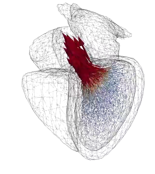
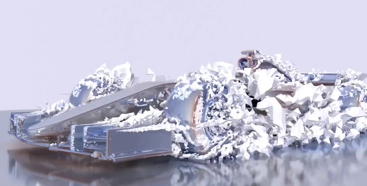
Contact: Johan Jansson jjan@kth.se
DigiMat is a spin-off of the Digital Math research environment: http://digitalmath.tech .
Kontakt: Johan Jansson jjan@kth.se
DigiMat är en spin-off från forskningsprojektet Digital Math: http://digitalmath.tech .

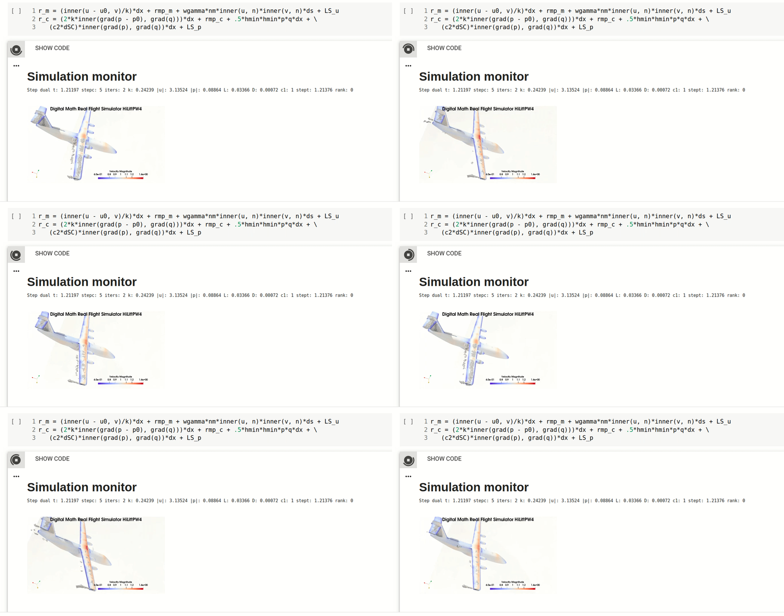
If you would like a certificate, e-mail Johan Jansson, jjan@kth.se, to learn more.
Om du vill ha ett certifikat — maila Johan Jansson, jjan@kth.se, för att veta mer.
In response to the current pandemic students and faculty at edX 40 partner universities now have the possibility to get a free coupon code to use to enroll to a verified track of this course.
To receive a coupon, you need to fulfill these requirements:
1) be a student or faculty at edX 40 partner universities
2) contact the MOOC team at your university, using your university e- mail account
3) write clearly what course you are interested in taking
Students and faculty at KTH contact moocx@kth.se
The coupons are valid until June 30th, 2020, and you have access to the course through the end of July.
How to use the code: enroll in the Verified Track, enter your enrollment code instead of a payment method, and start the course from the beginning. Codes are restricted to use by learners with a university email tied to their edX account. Learners who do not have a university email attached to their account will need to update their email address, please find the instructions here.
This is the first course in a series of two courses in the Digital Math Program, meant to be followed in sequence:
This course
The follow-up course
HPFEM02.1x requires you to run parallel simulations. Access to an easy-to-use web-based supercomputing interface will be made available to carry out
This study guide will focus on HPFEM01.1x. The specific Study Guide for HPFEM02.1x will be part of the HPFEM02.1x pages.
There is a wealth of Digital Math material available for all ages and levels, to prepare you for these courses, and to allow you to learn more advanced methods and applications.
The Digital Math: MOOC-HPFEM courses are given as part of the ELISE project for electric aviation, the DigiMat project for creating motivation and learning with Digital Math, and the ENABLE project for modeling avdnaced metals together with leading European industrial partners.
The course is divided into 7 modules, each representing one core concept of the course:
The course is self-paced, so all the course material is available from the start of the course.
To learn the material in each module, we recommend:
We recommend to do modules 1-3 in order, the other modules can be done in any order. Each module is expected to take approximately 3 hours to work through.
The examination for a certificate is based on a Digital Portfolio that you continuously build during you learning - meaning that you collect and organize skills, methods, derivations, key results, etc. that you have learned during the course. A teacher will then assess your Portfolio in relation to the learning goals.
Automated grading is available in the course to assist and support learning, but the automated grading is not the final summative examination. You can collect the results from the automated grading in your Portfolio, and a teacher will then assess the entire Portfolio.
To get a certificate
On most automatically graded assignments you have 2 attempts. Exceptions are check boxes where only two options are possible, then you you only have 1 attempt.
Participants who take the audit track (that don't pursue a certificate) will not be graded.
You must behave with academic honesty and respect your fellow students. Please abide by the edX Terms of Service Honor Code.
The course is self-paced, and there will be no structured sessions together with teachers. However, the teachers will be present in the discussion forums during the first month of the course.
A teacher will assess your Portfolio in relation to the learning goals.
Computer/tablet/smartphone
Please note that some of the activities/assignments in the course might not be accessible on a tablet or smartphone. If you're working on a tablet or smartphone and find yourself having technical problems please try the assignment again on a computer.
Browser
Make sure you have the latest version of the browser you're using. Here is a list of the supported browsers.
Should you come across some technical issues turn to the
The edXs Demo course DemoX will show you how to take an edX course. You will learn how to navigate the platform, test different types of problem and other features, and get an insight on how grades work in edX.
If this is your first course on edX.org we recommend that you start by taking the Demo Course.
Should you have questions or doubts a good idea is to look through the edX Learners Guide.
To get help with the course, click the Discussion tab and post a question. To get help with a technical problem, click Help to send a message to edX Student Support.
It is appreciated if you take the time to introduce yourself in the forum under topic "Learner presentations". This helps to build a community around the course.
Goal: Automatically generate the program, mesh and solution from PDE/model (residual) and goal functional $M(U)$ (e.g. drag).
Basic Case ("Modern Scientific Paper"):
https://colab.research.google.com/drive/1FIMAmWB8MiyhhI5KVxL0tCv7sYaYKsdt?usp=sharing
3D cube case:
After this session you should be able to:
Explain the piecewise linear approximation of a function, such as the solution in FEM, including mesh and cell size in the mesh.
Explain the piecewise linear approximation in terms of basis functions in a function space, conceptually and in FEniCS.
Explain the L2 inner product, and the associated L2 norm of functions, conceptually and in FEniCS.
Formulate L2 orthogonal projection using the L2 inner product, compute examples in FEniCS and compare against interpolation.
Solving complex PDE such as flow in heart or aerodynamics of aircraft requires systematic representation of the solution, such as 3D velocity field. This is what we will now learn about in this module
Define a computational domain, and then “triangulate” into “cells”, in 1D: intervals, in 2D: triangles, in 3D: tetrahedra [plot]. The “cell size” h is the diameter of a cell. $x_i$ are numbered “vertices” in the mesh.
Piecewise linear approximation of the function on the mesh - systematic representation - simple functions locally, pieced together into a complex function globally.
Represent the piecewise linear functions using basis functions - using the vector space concept from linear algebra in $R^n$
We can then define L2 inner product of functions, with associated norm and orthogonality - the key to FEM.
Based on these concepts we can formulate L2 projection - optimal piecewise linear representation of given function. We prove that L2 projection is the best possible approximation and compute examples to verify this. FEM is a generalization of L2 projection.
We want to approximate a known function $f(x)$.
Define piecewise linear (PWL) function approximation $U = U(x)$ as linear combination of simple “basis” functions $\phi_j(x)$: \[\begin{aligned} U(x) &= \sum_{j=1}^N \xi_j \phi_j(x)\end{aligned}\] Basis functions are in the vertices $x_j$ defined by: \[\begin{aligned} \phi_j(x) = \begin{cases} 1, &x = x_j\\ 0, &x \neq x_j \end{cases}\end{aligned}\]
and vary linearly between the vertices.
1D mesh of domain $\Omega = [0, 1]$ with cell size $h=0.1$, PWL function approximating $f(x) = 1 + \sin(10 x)$ as linear combination of basis functions $\phi_j(x)$ (right).
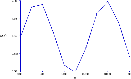
PWL function $U(x)$
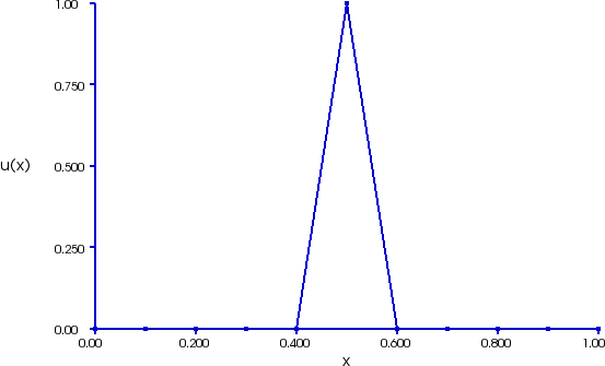
Basis function $\phi_j(x)$
The basis functions behave just like basis vectors in $R^n$, and form a “vector space of functions” or “function space” in short, which we call $V_h$.
This allows us to define an inner product of functions, the L2 inner product: \[\begin{aligned}(v, w) &= \int_\Omega vw dx\end{aligned}\] This in turn gives us the concept of orthogonality of functions, when the inner product is zero: \[\begin{aligned} (v, w) &= 0\end{aligned}\] and it generates the L2 norm, which allows us to measure the “size” of a function: \[\begin{aligned} \|v\|_{L_2} &= \sqrt{ \int_\Omega v^2 dx }\end{aligned}\]
We are now ready to formulate the basic mechanism of FEM - here in the form of an optimal orthogonal projection of a function into the FE function space, the optimal PWL approximation.
We cannot represent a given function $f(x)$ exactly as a PWL function: \[\begin{aligned} U(x) - f(x) &= 0 \end{aligned}\] the best we can do is require the residual, here the difference, to be orthogonal to the FE function space - or all basis functions: \[\begin{aligned} (U - f, v) = 0, \quad \forall v \in \{\phi_0, ..., \phi_N\} \end{aligned}\] v “test function”. Residual $R(U) = f - U$.
This is called the Galerkin Orthogonality.
Plot the reference $f(x)$, L2 projection and interpolation as comparison. The L2 norm of the projection error is about half that of the interpolation error. We will formally show that the L2 projection is the best possible approximation. Intuitive interpretation is that the projection is better in an “average sense”.
L2 projection $U(x)$ of the given function $f(x) = 1 + sin(10 x)$.
We will now formally show that FEM, here in the form of L2 projection, gives the best possible PWL approximation. The error $f - U$ is measured in the L2 norm $\|f - U\|_{L_2}$.
We will use the Cauchy-uSchwartz inequality for functions $v$ and $w$: \[\begin{aligned} (v, w)_{L_2} \leq \|v\|_{L_2} \|w\|_{L_2} \end{aligned}\] which has the same form as for vectors in $R^n$:
The proof of optimality is as follows: \[\begin{aligned} &\|f - U\|^2_{L_2} = (f - U, f - U) = {\color{blue}[\text{add:}\ 0 = v - v,\ \forall v \in V_h]} = \nonumber\\ &(f - U, f - v) + (f - U, v - U) = {\color{blue}[\text{use GO:}\ (f - U, v - U) = 0]} = \nonumber\\ &(f - U, f - v) \leq {\color{blue}[\text{use Cauchy-Schwartz}]} \leq \|f - U\|_{L_2} \| f - v \|_{L_2}\\ &\Rightarrow \nonumber\\ &\|f - U\|_{L_2} \leq \| f - v \|_{L_2},\ \forall v \in V_h \end{aligned}\]
This means that the error for the FEM solution $U$ is smaller than the error for any other PWL function $v$ (for example interpolation), i.e. $U$ is the best possible PWL approximation. From the proof we see that this is because $U$ satisfies the Galerkin Orthogonality.
expression for $f(x)$, PWL function space, test function, inner product and L2 projection, compact solve interface.
from dolfin import *

mesh = UnitIntervalMesh(6)
V = FunctionSpace(mesh, "CG", 1)
f = Expression("1 + sin(10*x[0])", degree=5)

# L2 projection
U = Function(V)
v = TestFunction(V)
r = inner(U - f, v)*dx
solve(r == 0, U)

# Comparison to interpolation
If = interpolate(f, V)After this session you should be able to:
In this module we will focus on goal-oriented adaptive error control.
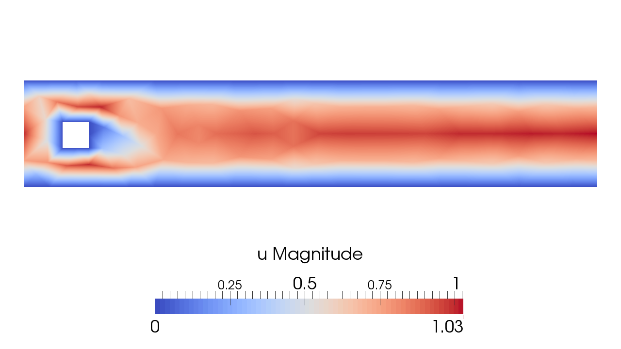
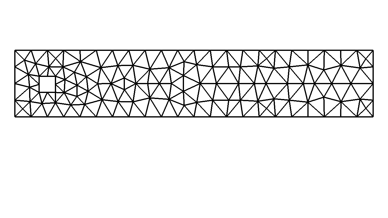
$ |M(e)| \le TOL \Rightarrow$
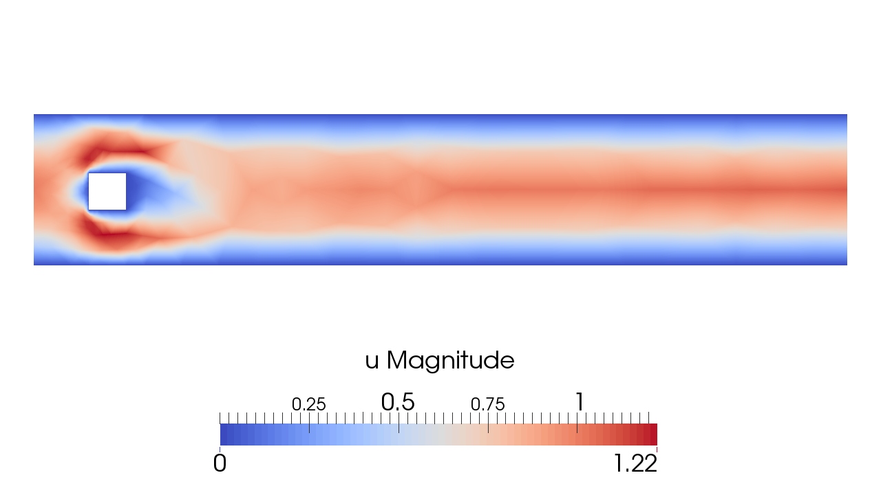
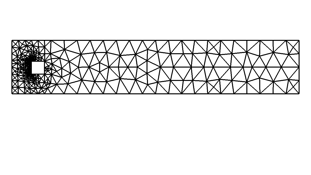
with $M(e)$ a “goal functional” (e.g. the drag force) of the computational error $e = u - U$.
We give a “starting mesh” as a guess, and based on a computable “a posteriori error estimate”that we will derive, we iteratively solve the problem $r(U, v) = 0$ and refine the mesh to satisfy a given tolerance on the error.
Goal quantity Force $F$:
$F = \frac{1}{|I|} \int_I \int_{\Gamma_a} pn \, ds dt$, $\Gamma_a$ boundary of aircraft, $p$ the pressure, n normal.
We derive the “error representation” which tells us where in the domain the error contribution is large: $M(\hat{e}) = -r(\hat{U}, \hat{\phi})$
(NB! residual $r$ computable!)
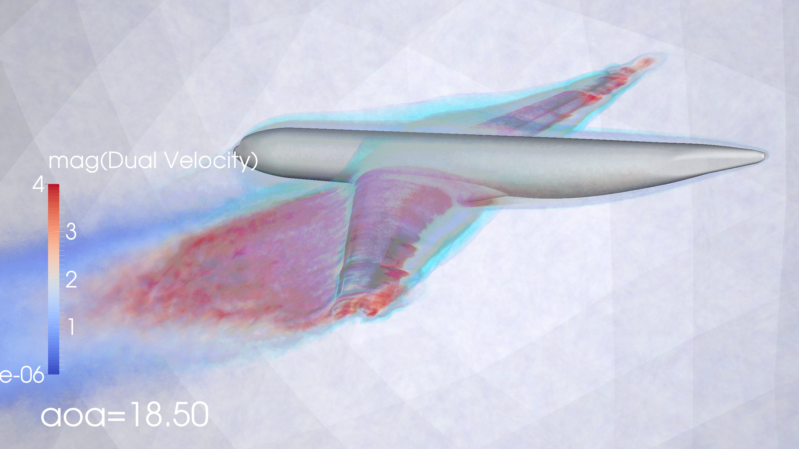
Adjoint velocity $\hat{\phi}$

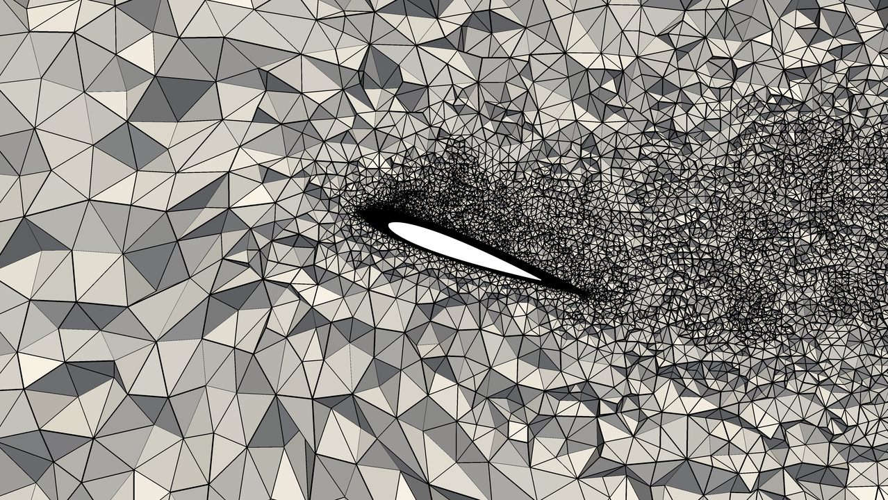
Coarse starting mesh
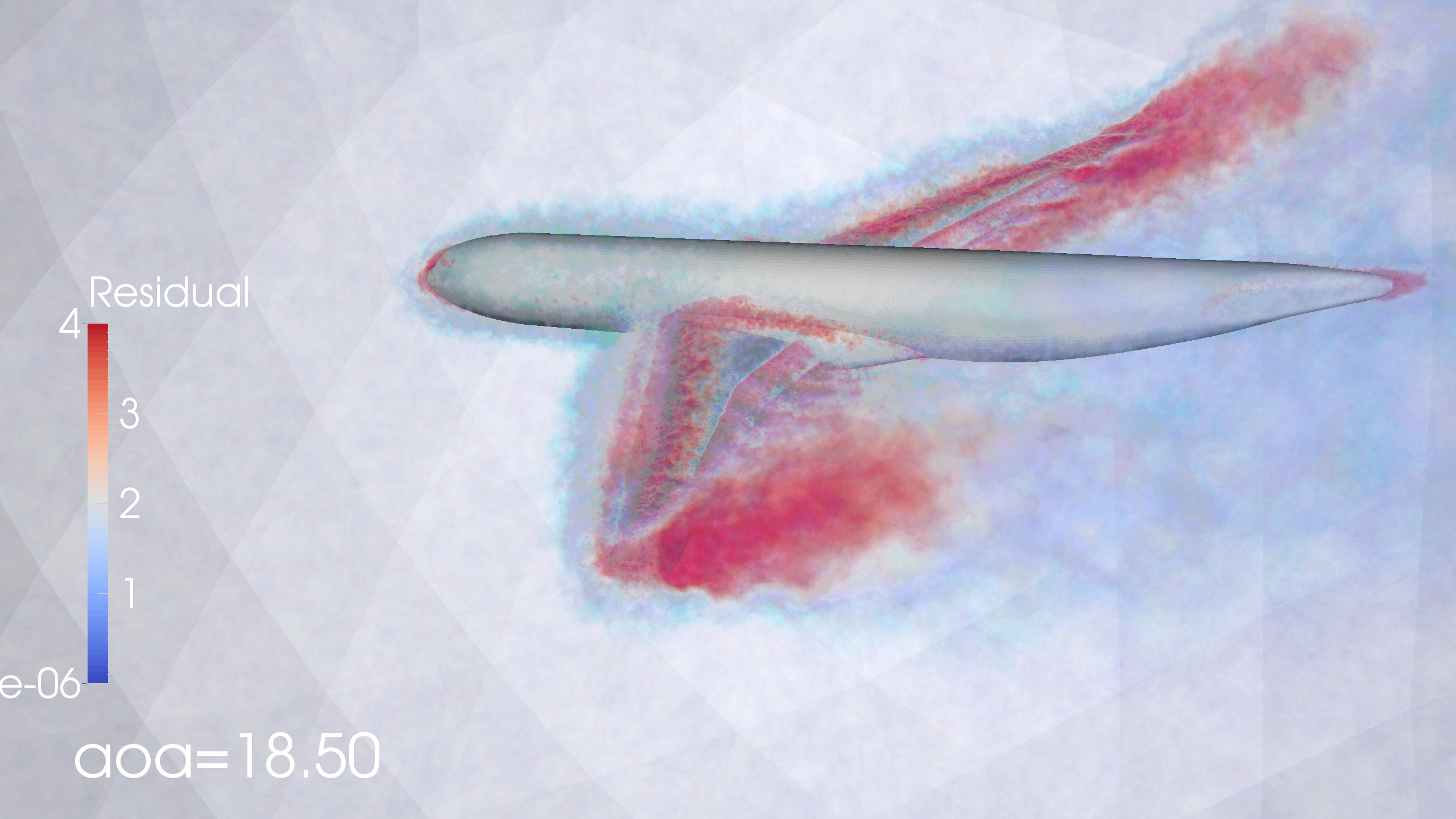
Residual $R(\hat{U})$
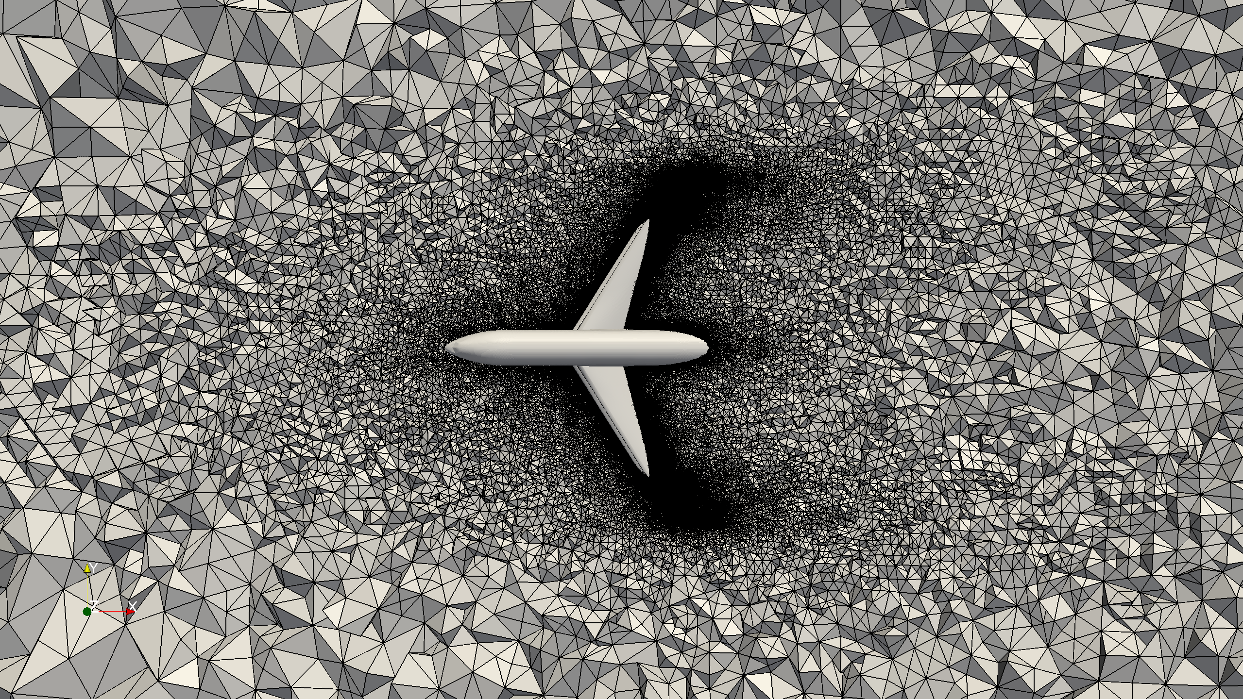
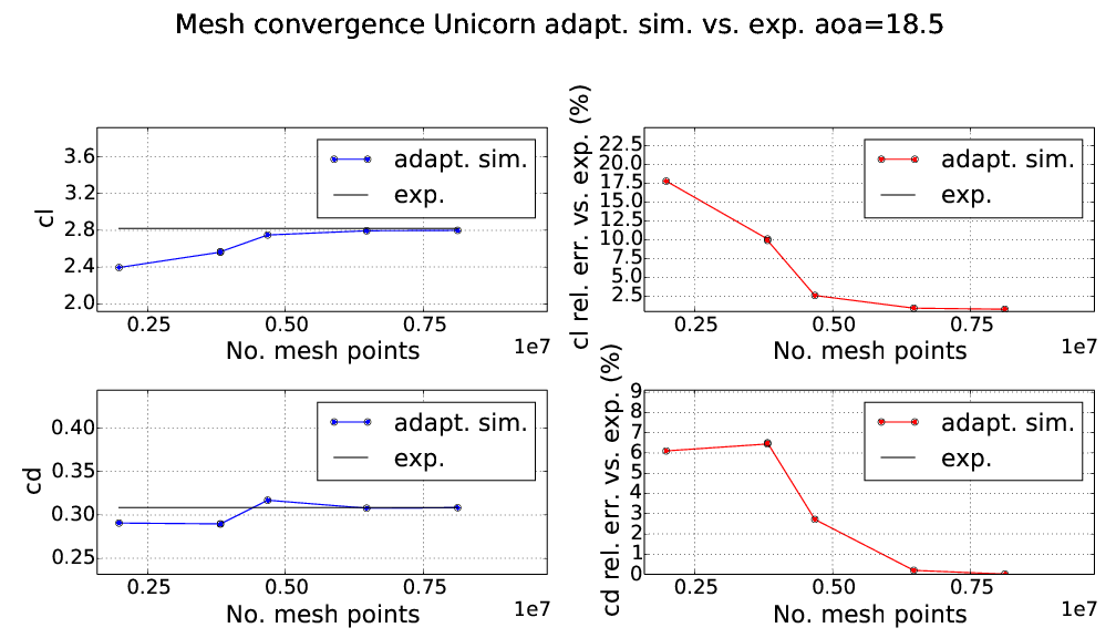
Refined mesh 5 adapt. it.
Lift and drag within 1.5% of exp.
Use 1280 cores on SuperMUC supercomputer
For a linear problem in weak residual formulation: \[\begin{aligned} r(u, v) = 0 \end{aligned}\] we introduce the adjoint problem for the adjoint solution $\phi$: \[\begin{aligned} r(v, \phi) = M(v) \end{aligned}\] where we simply have switched order of the test and trial functions $u$ and $v$.
We then have for the error $e = u - U$: \[\begin{aligned} M(e) = r(e, \phi) = r(u, \phi) - r(U, \phi) = -r(U, \phi) \end{aligned}\] We note that the approximate solution U is computable, and given the adjoint $\phi$ we can exactly compute the error. We typically compute an approximation $\Phi$ to give us an error estimate.
We can decompose the error representation into a sum over all cells: \[\begin{aligned} M(e) = -r(U, \phi) = \sum_{K \in T} r(U, \phi)_K \end{aligned}\] The “error indicator” ${\cal E}_K$ for cell K is then: \[\begin{aligned} {\cal E}_K = |r(U, \phi)_K| \end{aligned}\] By refining the cells with largest indicator, we optimally reduce the error.
Due to the Galerkin orthogonality, $r(U, \Phi) = 0$ if $\Phi, U \in V_h$, however, the local error indicator $r(U, \Phi)_K$ is not zero, and carries information about the local error contribution.
Do-nothing adaptive algorithm
Choose an initial triangulation $T_h^0$ as starting guess.
Compute FEM solution $U$ on $T_h^j$
Evaluate stopping criterion, either the error representation: \[\begin{aligned} |r(U, \Phi)| \leq TOL \end{aligned}\] if available, or the goal quantity from two successive adaptive iterations: \[\begin{aligned} |M(U^j) - M(U^{j-1})|| \leq TOL \end{aligned}\]
Refine a percentage of cells $K$ where the error contribution/indicator ${\cal E}_K = |r(U, \phi)_K|$ is largest, with local mesh bisection (e.g. Rivara refinement for simplices).
for i in range(0, maxiters): # Adaptive loop
        # Solve primal eq. given r
        solve(r==0, U)

        # Construct+solve adjoint eq.
        a_adj = adjoint(derivative(r, U)) # differentiate to get lhs
        L_adj = goal(v) # goal quantity as rhs
        solve(a_adj==L_adj, Phi, bc)

        # Construct error representation
        r = replace(r, {v: z*Phi}) # z pw constant test function

        # Compute error indicators
        ei.vector()[:] = assemble(r).array()

    # Mark cells for refinement and refine
    gamma = abs(ei.vector().array())
    cellmarkers = MeshFunction("bool", mesh, mesh.topology().dim())
    gamma_0 = sorted(gamma, reverse=True)[int(len(gamma)*adapt_ratio) - 1]
    for c in cells(mesh):
      cellmarkers[c] = gamma[c.index()] > gamma_0
mesh = refine(mesh, cellmarkers)Welcome to the course part "High Perfomance FEM I". In this part of the course you will get an overview of the course and learn about performance in an adaptive FEM and HPC setting. The learning outcomes for this part are:
Define the concepts of performance, scalability, computational cost, accuracy in the setting of FEM and turbulent flow.
Describe a distributed-memory architecture and the message passing programming model.
Estimate the performance of different parallel algorithms, such as adaptivity, efficient time-stepping.
Describe the process of mesh partitioning and the distributed mesh data structure including ghost entities.
Describe how methods for solving linear system are influenced by distributed data structures.
Give an overview of the Direct FEM methodology and FEniCS-HPC
Describe how to carry out FEniCS-HPC simulations of turbulent flow on a supercomputer.
Analyze the performance benefit of taking large timesteps in a parallel setting.
Analyze the performance benefit of adaptivity.
What is performance? Fast? Cheap? Scalable? Accurate?
Modern computers - parallel architectures

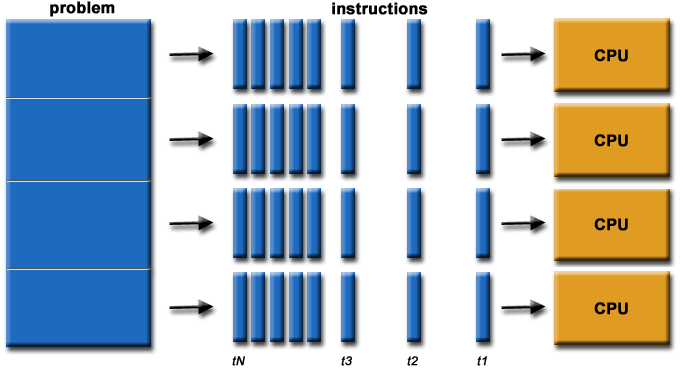
$N_{PE}$ - number of Processing Elements (PE), e.g. CPU cores.
Distributed architecture: each PE has its own memory
Network communication is expensive - computation is cheap.
Parallel and distributed computing in FEniCS-HPC
Distributed meshes and matrix-vector operations
FEniCS-HPC programming interface
Efficient solution of turbulent flow
We have derived general FEM for solving time-dependent PDE models in weak residual form: \[\begin{aligned} r(U, v) = 0, \quad U \in I \times V_h \quad \forall v \in I \times V_h \end{aligned}\]
With the derived automation algorithms realized in FEniCS we can automatically generate implementations and compute solutions with adaptive error control to satisfy a bound on the error:
\[\begin{aligned} |M(e)| < TOL \end{aligned}\]
We want our computations to be:
Fast wall-clock time $T_W$ (“time to solution”).
Cheap resource utilization, $C_{cost} = N_{PE} \, T_W$.
Guarantee an error bound $M(e) < TOL$
Constant $C_{cost}$ vs. $N_{PE}$ (2x $N_{PE}$ $\Rightarrow$ $\frac{1}{2}$ $T_W$)
Linear growth in the number of unknowns $T_W = O(N_{DOF})$
We achieve low $C_{cost}$ vs. error $|M(e)|$ and realiability by efficient and robust mathematical methods - adaptivity and large timesteps
We achieve high strong scalability by efficient use of the hardware - optimizing communication
We achieve scalable methods by exploiting sparse linear algebra.
For a time-dependent problem the total wall-clock time $T_W$ is the sum of the wall-clock time of all the time steps:
$T_W = \sum_{i=0}^N T_k$
The timestep size is restricted by:
$k < C_{CFL} min(\frac{h}{|U|})$
$|M(e)| < C_k k^p$
For many methods, the stability restriction dominates.
In module TBD we describe a method for allowing significantly larger timesteps, allowing a direct reduction of $T_W$ $\Rightarrow$ significant improvement of efficiency and effectiveness.
The presented adaptive method optimizes the error $|M(e)|$ vs. $N_{DOF}$, giving high efficiency and effectivity.
Standard for communication between the local memory of processing elements (PEs) on parallel architectures
Suitable for distributed memory architectures
Message passing
Send and receive
Blocking and non-blocking communication
Collective communication
Communication is expensive - do as much work as possible locally and communicate only when needed
Recall the FEM problem:
Find $U \in V_h$ such that
\[r(U,\, v) = 0, \quad \forall v \in V_h,\]
A linear problem, or linearization can be written as:
\[a(U,\, v) = L(v), \quad \forall v \in V_h,\]
where $V_h$ is a finite dimensional function space on the domain $\Omega$.
Testing against the basis $\{\varphi_i\}_{i=0}^n$ of $V_h$ leads to a system of linear equations
\[A \xi = b,\]
where the matrix $A = A_{ij} = a(\varphi_j, \, \varphi_i)$.
How to solve this efficiently on a parallel architecture?
$A$ assembled by summing the contributions from each element $K \in \mathcal{T}$, where $\mathcal{T}$ (the mesh) is a partitioning of $\Omega$
Each PE responsible for assembly over a subset of the elements $K \in \mathcal{T}$
Communication or synchronization is required on the boundary between two partitions
assemble $A^K$
$A_{\mathcal{I}(i)\,\mathcal{I}(j)} = A_{\mathcal{I}(i)\,\mathcal{I}(j)} + A_{ij}^K$
Data needed for local assembly is available on each PE
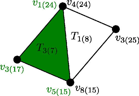
Vertices are shared at the boundary between mesh partitions
Data dependency at shared vertices on update of global matrix $A$
A shared vertex is owned by one PE and stored as a ghost vertex on the other PEs that share the vertex
Developed over a 20+ year period by Johnson, Hoffman, Jansson, etc.
Incompressible Euler as model for high Reynolds number flow, such as flight: \[\begin{array}{rcll} R(\hat{u}) &=& \begin{cases} p_t u + (u\cdot \nabla) u + \nabla p = 0\\ \nabla \cdot u = 0 \end{cases}\\ u\cdot n &=& 0, x \in \Gamma \quad (\text{Slip BC})\\ \hat{u} &=& (u, p) \end{array}\]
Weak residual $r(\hat{u}, \hat{v}) = (R(\hat{u}), \hat{v})$
\[\begin{aligned} &r(\hat{U}, \hat{v}) = (R(\hat{U}), \hat{v}) + (\delta R(\hat{U}), R(\hat{v})) = 0\\ &\delta = h, \, \forall \hat{v} \in \hat{V}_h, \, \hat{U} \in \hat{V}_h\end{aligned}\]
Directly use error representation: $\quad M(\hat{e}) = r(\hat{U}, \hat{\phi})$
Error indicator: ${\cal E}_K = r(\hat{U}, \hat{\phi})_K$
[Hoffman, Jansson, et. al., 2012 C&F], [Hoffman, Jansson, et. al. 2016, Encyclopedia of Computational Mechanics]
Automated generation of finite elements/basis functions ( FIAT) \[e = (K, V, \mathcal{L})\]
Automated evaluation of variational forms on one cell based on code generation ( FFC+UFL) \[A^K_{ij} = a_K(\phi_i, \phi_j) = \int_K \nabla \phi_i \cdot \nabla \phi_j dx = \int_K lhs(r(\phi_i, \phi_j) dx)\]
Automated parallel assembly+solve of discrete systems on a distributed mesh $\mathcal{T}_{\Omega}$ (w/ refinement) using PETSc/JANPACK as sparse LA backends ( DOLFIN-HPC)
5cm
$A = 0$
for all cells$K \in \mathcal{T}_{\Omega}$
$A$+=$A^K$
$Ax = b$
Automated adaptive turbulent Unified Continuum modeling ( Unicorn)
\[r_{UC}((v, q), (u, p)) = (v, \rho (\partial_t u + (u \cdot \nabla) u) + \nabla \cdot \sigma - g) + (q, \nabla \cdot u) + LS((v, q), (u, p))\]
Aim: Automate as much as possible (as little hand-written code as possible)
Components connected in minimal C++ program: time-stepping and fixed-point iteration loop, coefficients
# Strong residual + GLS stabilization
R = [grad(p) + grad(um)*um, div(um)]
R_v = [grad(v)*um, div(v)]
R_q = [grad(q), 0]

LS_u = d*(sum([inner(R[i], R_v[i]) for i in range(0, 2)]))
LS_p = d*(sum([inner(R[i], R_q[i]) for i in range(0, 2)]))

# Weak residual for stationary equation
rs_m = (nu*inner(grad(u), grad(v)) + inner(grad(p) + grad(u)*u, v))*dx
rs_c = (inner(div(u), q))*dx

# Evaluate residual at midpoint (in time)
um = 0.5*(u + u0)
rmp_m = replace(rs_m, { u: um })
rmp_c = replace(rs_c, { u: um })

# cG(1) timestepping method with segregated fixed-point iteration + Schur precond.
r_m = (inner(u - u0, v)/k)*dx + rmp_m + LS_u*dx
r_c = (alpha*inner(grad(p - p0), grad(q)))*dx + rmp_c + LS_p*dx
With the presented DFS methodology and FEniCS HPC framework you will be able to carry out prediction of gross quantities in turbulent flow, such as flight dynamics.
Welcome to the course part Real Flight Simulation. In this part of the course you will get an understanding of the mechanism of flight and how to efficiently compute flight simulation with Direct FEM. After this session you should be able to:
After this session the student should be able to:
Describe the mechanism of flight in the setting of DFS, including drag, lift, separation and stall.
Perform DFS simulations of high Re aerodynamics and flight, comparing to experimental references.
Analyze the performance of DFS based on the grand-challenge problem of flight-simulation, comparing to other simulation techniques.
DFS enables high Reynolds number aerodynamics sim. at high efficiency by:
Adaptive error control
Large time steps
Slip wall model with 3D slip-separation mechanism.
DFS and Unicorn/FEniCS-HPC enables:
Time-dependent simulation of aircraft in few hours - weeks using standard methods [Löhner].
Easy understanding of mechanism of flight.
Developed over a 20+ year period by Johnson, Hoffman, Jansson, etc.
Incompressible Euler as model for high Reynolds number flow, such as flight: \[\begin{array}{rcll} R(\hat{u}) &=& \begin{cases} p_t u + (u\cdot \nabla) u + \nabla p = 0\\ \nabla \cdot u = 0 \end{cases}\\ u\cdot n &=& 0, x \in \Gamma \quad (\text{Slip BC})\\ \hat{u} &=& (u, p) \end{array}\]
Weak residual $r(\hat{u}, \hat{v}) = (R(\hat{u}), \hat{v})$
\[\begin{aligned} &r(\hat{U}, \hat{v}) = (R(\hat{U}), \hat{v}) + (\delta R(\hat{U}), R(\hat{v})) = 0\\ &\delta = h, \, \forall \hat{v} \in \hat{V}_h, \, \hat{U} \in \hat{V}_h\end{aligned}\]
Directly use error representation: $\quad M(\hat{e}) = r(\hat{U}, \hat{\phi})$
Error indicator: ${\cal E}_K = r(\hat{U}, \hat{\phi})_K$
Aim: Automate as much as possible (as little hand-written code as possible)
Components connected in minimal C++ program: time-stepping and fixed-point iteration loop, coefficients
# Strong residual + GLS stabilization
R = [grad(p) + grad(um)*um, div(um)]
R_v = [grad(v)*um, div(v)]
R_q = [grad(q), 0]

LS_u = d*(sum([inner(R[i], R_v[i]) for i in range(0, 2)]))
LS_p = d*(sum([inner(R[i], R_q[i]) for i in range(0, 2)]))

# Weak residual for stationary equation
rs_m = (nu*inner(grad(u), grad(v)) + inner(grad(p) + grad(u)*u, v))*dx
rs_c = (inner(div(u), q))*dx

# Evaluate residual at midpoint (in time)
um = 0.5*(u + u0)
rmp_m = replace(rs_m, { u: um })
rmp_c = replace(rs_c, { u: um })

# cG(1) timestepping method with segregated fixed-point iteration + Schur precond.
r_m = (inner(u - u0, v)/k)*dx + rmp_m + LS_u*dx
r_c = (alpha*inner(grad(p - p0), grad(q)))*dx + rmp_c + LS_p*dxSlightly viscous bluff body flow such as flight can be viewed as zero-drag/lift potential flow modified by 3d slip separation instability of potential flow, into turbulent flow with nonzero drag/lift.
In this course you will have opportunity to carry out Detailed adaptive DFS in FEniCS-HPC branch validating the theory for wings/full aircraft + several other model and complex problems.
Force: $F = \frac{1}{|I|} \int_I \int_{\Gamma_a} pn \, ds dt$,
with $\Gamma_a$ surface of aircraft/wing and $p$ the pressure
Drag and lift coeff.: $c_d = \frac{2 F_0}{|\bar{u}|^2 A}$, $c_l = \frac{2 F_1}{|\bar{u}|^2 A}$,
with $A$ reference area of aircraft/wing and $\bar{u}$ freestream/inflow velocity
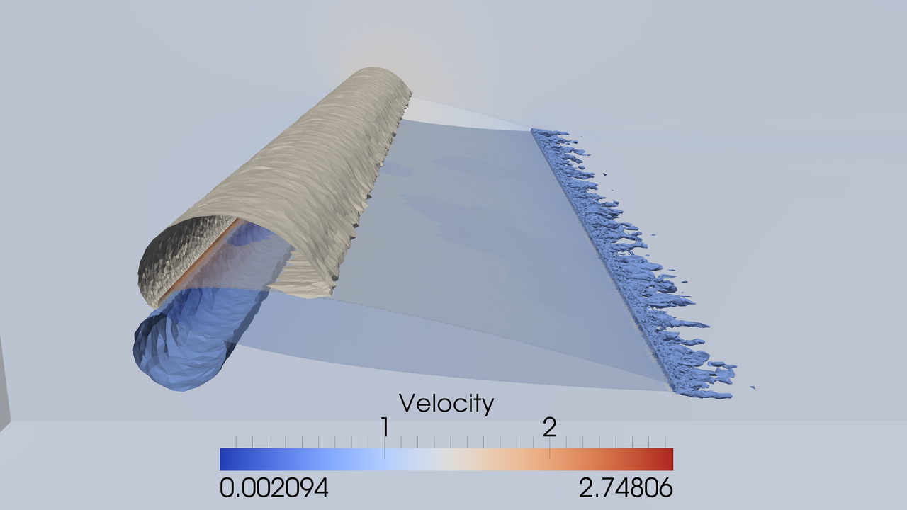
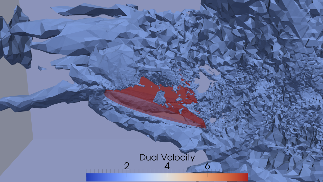
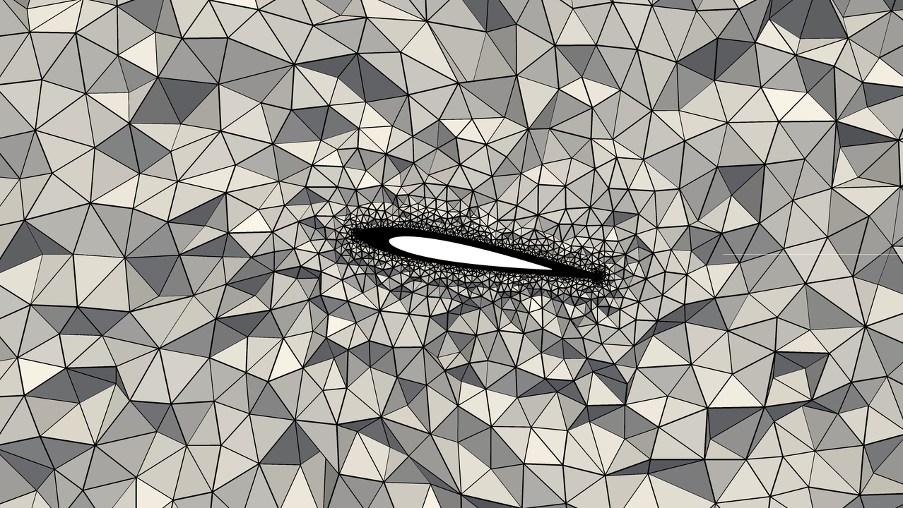
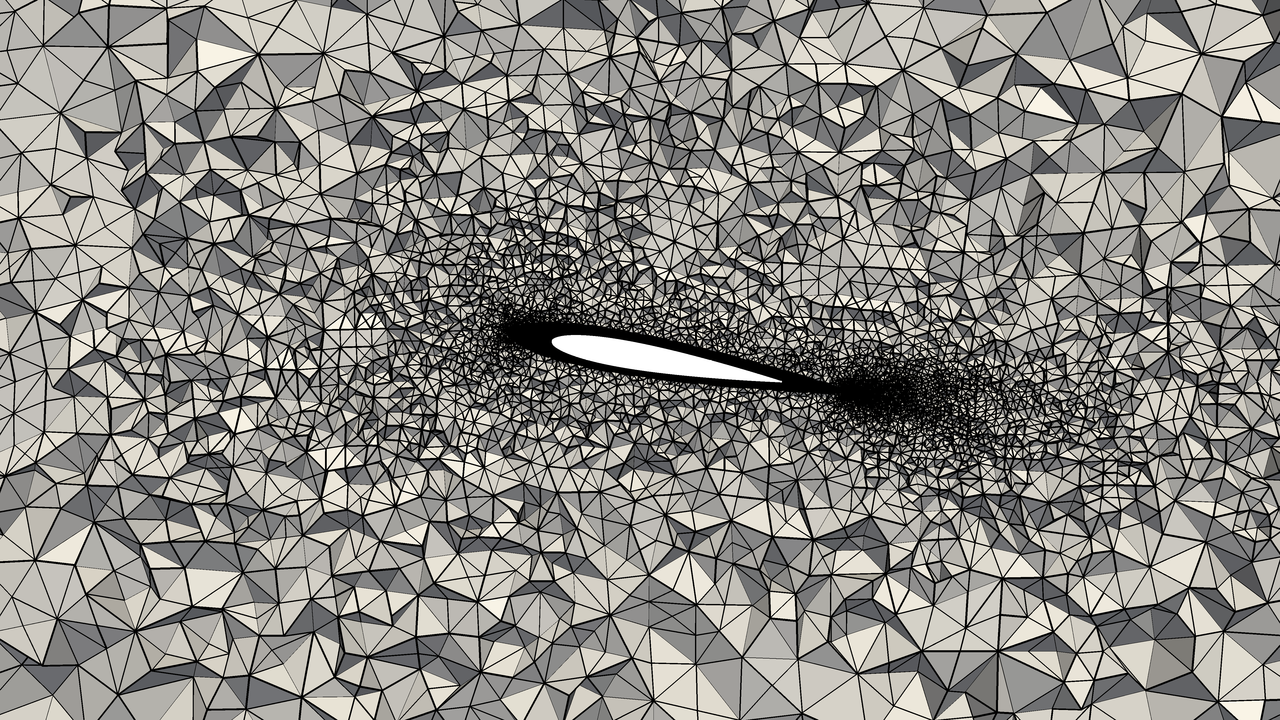
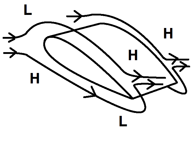
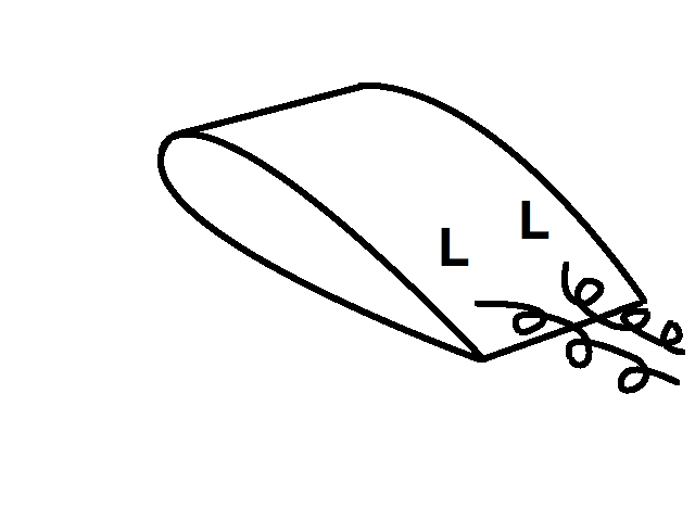
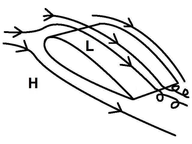
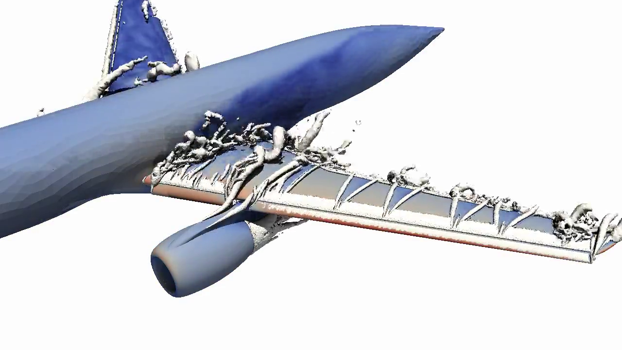
Note slip separation at rounded trailing edge.
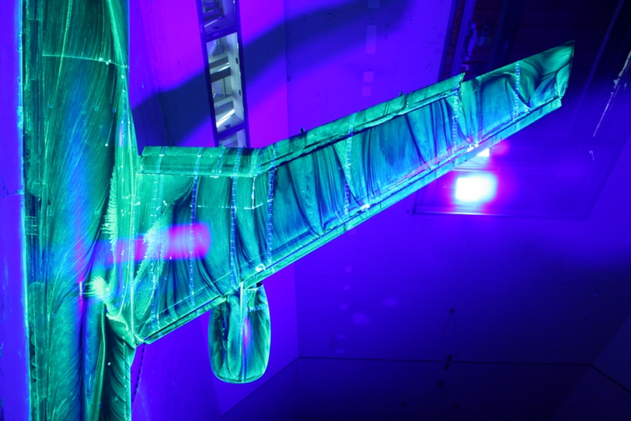
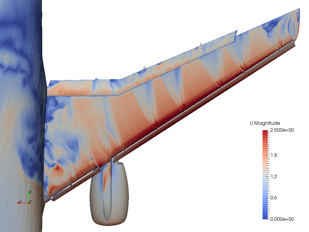
Surf. vel. exp. $\alpha=21.57$ and sim. $\alpha=22.56$
JSM pylon-on, $\alpha=22.56$, wing B-B
No trip-force (unstalled)
With trip-force (stalled)
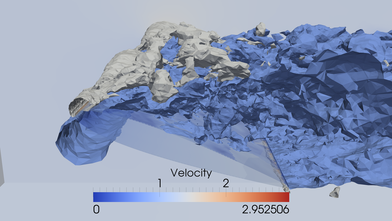

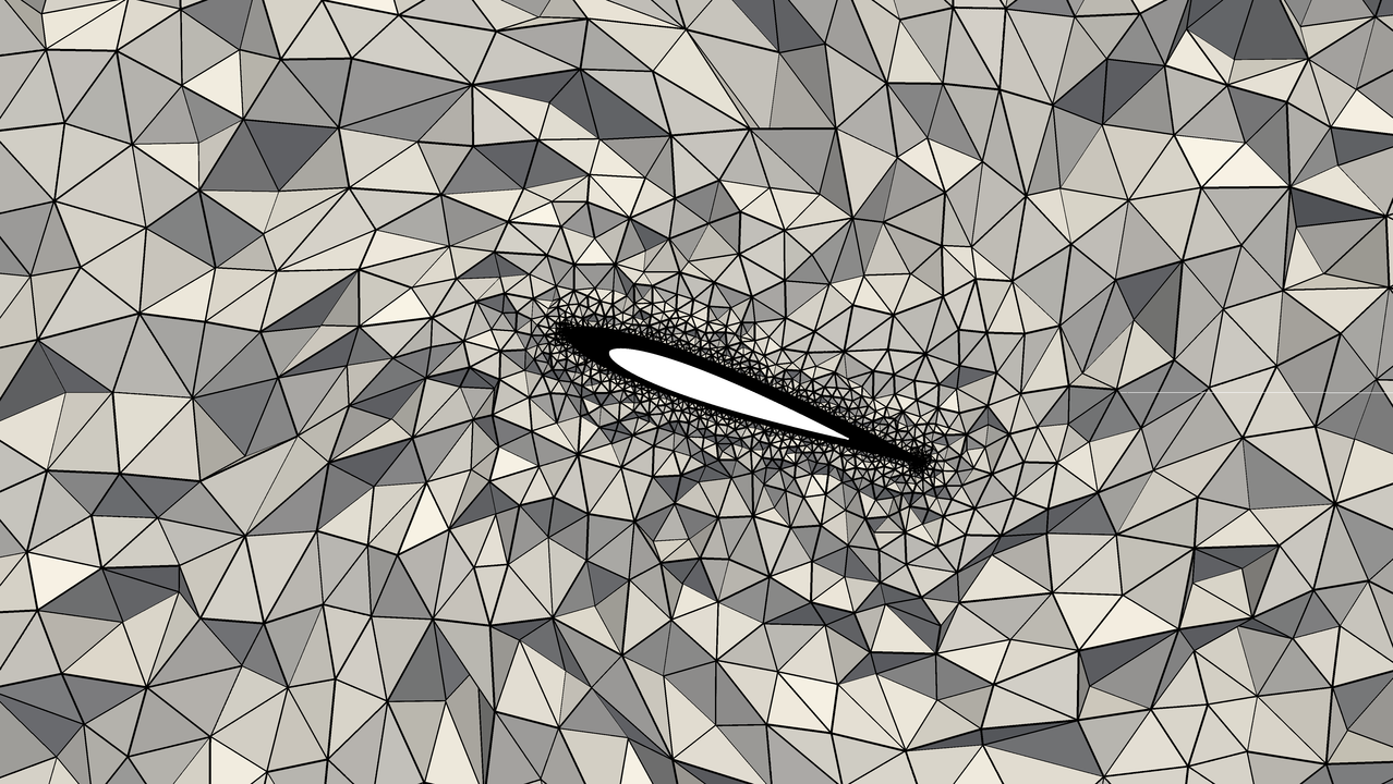
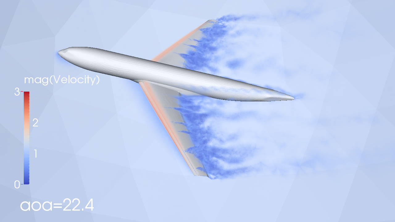
For higher angle of attack we observe stall, flow separates at leading edge, removes low pressure “suction” at leading edge, gives large drag from large wake. [Hoffman, Jansson, Johnsson, JMFM, 2015]
DFS enables high Reynolds number aerodynamics sim. at high efficiency by:
Adaptive error control - uniform refinement grows as $N_{DOF} \propto h^{-3}$ - refining once increases $N_{DOF}$ by 8x. Adaptivity allows minimal $N_{DOF}$ - on the order of resolving the geometry for 5% accuracy, ca. $10^6 \ N_{DOF}$
Large time steps - 100-1000 larger time steps than standard methods [PyFR]
Slip wall model - enormous efficiency gain by avoiding having to resolve a thin boundary layer of cost $\approx Re^2 \approx 10^{16} N_{DOF}$ which is impossible even for largest supercomputers today.
Mathematical programming unifies math and coding. It’s based on scientifically grounded physics simulations, which means computing and predicting scenarios with a computer. With DigiMat you’ll learn to create your own virtual worlds.
DigiMat is for everyone, no matter age or level. Kids, parents, teachers and university students and professionals. Anyone can learn to use the simple algorithms of DigiMat.
Mathematical Programming is crucial for industry and our digital society. With mathematical programming you can do much more powerful, interesting and useful things than with regular coding.
DigiMat focuses on motivation, creativity and learning by doing. Motivation is key to store information in the long term memory. By focusing on the amazing things you can achieve you'll find motivation to learn more and reach higher.
With mathematical programming you get a better understanding of the algorithms rather than learning special cases by heart, which is what traditional math education often focus on. You learn that the basics of math and coding are the same, and by that you understand the basic principles of both mathematics and programming.
Matematisk programmering förenar matte och kodning och bygger på vetenskapligt grundad fysiksimulering. Det betyder att du kan förutsäga fysiska händelseförlopp med hjälp av en dator. Du kan — i datorn — få flygplan att flyga, hjärtan att slå och skapa artificiell intelligens.
DigiMat är för alla, oavsett ålder, intresse eller förkunskaper. Barn, vuxna, föräldrar, lärare, universitetsstudenter och professionella har nytta och glädje av DigiMat. Alla kan lära sig de enkla algoritmer som DigiMat bygger på.
Därför att Matematisk programmering är avgörande för industrin och vårt digitala samhälle. Att kunna förutsäga skeenden och testa idéer digitalt är avgörande för all design och ingenjörskonst. Med matematisk programmering kan du göra långt mer kraftfulla, intressanta och användbara saker än med vanlig kodning. Ditt barn blir mer motiverad att lära sig matte och kodning, och du själv blir mer intressant på arbetsmarknaden.
DigiMat förenar matte och kodning och utgår från fysiksimulering, vilket inga andra aktörer gör. Du lär dig också avancerade algoritmer samtidigts om inga förkunskaper krävs. Även den lekfulla och kreativa pedogiken i kombination med högkvalificerad matematik gör DigiMat ensamt i sitt slag. Med den unika DigiMat-appen kan du skapa fritt och snabbt se resultat, det händer grejer och och är kul att hålla på med redan första gången du provar.
DigiMat fokuserar på motivation, kreativitet och att lära sig genom att göra. Det är faktorer som är avgörande för långsiktigt lärande, enligt pedagogisk forskning. Självklart krävs det tid och övning för att lära sig något och DigiMat är ingen quickfix. Men vårt mål är att du ska bli så motiverad och ha så kul att du inte vill göra annat än att lära dig mer.
I DigiMat Basic används Javascript, eftersom alla har tillgång till det i webbläsaren, och på avancerad nivå används Python. DigiMat begränsar dig dock inte till bara dessa språk, utan du lär dig algoritmerna och principerna som gäller för de flesta kända programmerings-språk.
Ja DigiMat täcker läroplanen och sträcker sig ännu längre. Den traditionella matematikundervisningen idag är till stor del föråldrad och baserad på hur det såg ut innan datorn fanns. DigiMat är modern, digitalt baserad matematik som kompletterar den traditionella undervisningen.
Du ska som lärare enkelt ska kunna använda DigiMat i undervisningen, utan att först behöva gå kurser eller ägna dig åt tidskrävande förberedelser. Du har bland annat hjälp av korta instruktionsvideor som kan visas i klassrummet och som steg för steg förklarar roliga och meningsfulla läraktiviteter.
